Ever got confused by difference between the two GLMs? With why ANCOVA and GLM do the same thing? Ever had trouble remembering assumptions? Stop thinking in tests and start thinking in mathematical models, and everything will be much clearer.
Math can be complicated, but it also simplifies talking about complicated concepts. The clearest way to define is by writing down the equations. That gives no room for confusion about what type of model you are talking about.
Outline
Starting with the most general formulation of GLM (the generalized linear model), passing through the definition of the general linear model we will arrive at the familiar $y = mx+b$ of the simple linear model. We will also see how the linear model relates to ANOVA and ANCOVA. I will provide animations and examples on how to generate synthetic data conforming to each specific model. Playing around with such simulated data is a good way to understand how certain models behave, so I encourage you to change the parameters and see what happens. Finally, I will refer you to some further reading, as there’s an excellent, graphic summary of all things linear models.
Generalized linear models
Notation and variables
Let $Y$ be our dependent (or response) variable, while let $X$ be our independent (or explanatory) variable. In this writing, we will only have one response variable, but we might have several explanatory variables. In the latter case, I will index them as $X_a, X_b$, etc. Capital letters will denote the variable in a theoretical sense (as a random variable), while lowercase letters $y, x$ (or $x{a}, x{b}$, etc.) will denote actual measurements of that variable.
This distinction between the variable and its measurements is an important concept. The $Y$ response variable has a probability distribution, in most cases it has a mean and a variance. But if I measure it say three times I will get three distinct values of $y$, $y_1$, $y_2$, and $y_3$. These values can now be used to estimate for example the mean and variance of $Y$, or more generally, the distribution of $Y$. In fact, the entire concept of mathematical modeling is trying to figure out what the distribution of the response variable is, and how the explanatory variables influence this distribution.
The parameters of the models will be denoted by $\beta$’s. These are fix numbers, but we do not know them and must be estimated based on our data.
Formulating the GLM
With that out of the way, we can now formulate the generalized linear model as two equations:
\begin{equation}(Y \mid X = x) \sim f(x,\Theta(x))\end{equation}
\begin{equation}g(E(Y \mid X = x)) = \eta(x)\end{equation}
Conceptually, this is probably the hardest part, so let’s break this down carefully.
In Eq. 1 the right hand side and the left hand side is divided by the $\sim$ sign and it reads: $Y$, when $X$ is set to a specific value $x$, is drawn from the distribution on the right hand side. The right hand side is one of the probability distributions from exponential family of distributions. This is a big family, but includes the most common distributions, for example the normal (Gaussian) and the Poisson distributions.
$\Theta$ stands for all the parameters these distributions can have, like $\mu$ and $\sigma$ in the normal or $\lambda$ in the Poisson distribution. It’s written as $\Theta(x)$ to show that these parameters also change as $X$ changes.
The linear in the GLM comes from Eq. 2. Here $g$ is the so-called link function (more on this later, but this is usually a simple function like the logarithm or the identity function, i.e. the do nothing function), $E(Y \mid X = x)$ is the expected value (mean) of $Y$, when $X$ is set to a specific $x$, and $\eta$ is the linear predictor. $\eta$ is called that, because it is a linear combination.) of the explanatory variables. Think $\eta = \beta_a\cdot x_a + \beta_b\cdot x_b + \beta_0 $, where the $\beta$’s are parameters of the model and $X_a$ and $X_b$ are two explanatory variables.
I also wrote only one $X$, but there could be many more. In that case, each of them would be set to a specific value in the above equations.
But what does this mean?
Let’s look at simple examples, which we can actually visualize.
Example with normal distribution
Taking only one explanatory variable, we can set the simplest linear predictor as $\eta = \beta x + \beta_0$. We choose our distribution (Eq. 1, right hand side), to be the normal (Gaussian) distribution and the link function to be the identity function. This sets the left hand side of Eq. 2 as:
\begin{equation}g(E(Y \mid X = x)) = E(Y\mid X = x) = \mu(x) \end{equation}
thus from Eq. 2, with our simple $\eta$ we have $\mu(x) = \eta = \beta x + \beta_0$. Eq. 1, thus becomes
\begin{equation}(Y \mid X = x) \sim \mathcal{N}(\mu(x),\sigma) = \mathcal{N}(\beta x + \beta_0, \sigma)\end{equation}
where $\mathcal{N}(\mu,\sigma)$ is the usual way to denote a normal distribution with a mean of $\mu$ and a variance of $\sigma$. We can write it more simply by leaving off the given $X = x$ part:
\begin{equation}Y \sim \mathcal{N}(\beta x + \beta_0, \sigma)\end{equation}
To put it in words: if we fix the $X$ (say $X$ is the temperature and it doesn’t change) then the measurement $y$ of $Y$ will be drawn from the distribution $\mathcal{N}(\beta x + \beta_0, \sigma)$. If we change $X$, then we change the mean of this distribution, thus the distribution of $Y$ will also change. It also means that whatever the change in $X$, the $\beta$’s and $\sigma$ will stay constant. Actually, the latter is where the homoscedasticity assumption comes from in linear regression. From the form Eq. 5, the normality assumption for the residuals should also be readily apparent.
This is something we can now visualize. For each given $x$, the mean of $Y$ is a straight line, and the error on it is a normal distribution with a variance of $\sigma$. It also shows why $\beta_0$ is called the intercept: if you set $x=0$, the blue line will intercept the $y$ axis at $y = \beta_0$. Unless you are absolutely sure that your model (the blue line) goes through the origin ($x = 0$ and $y = 0$), always include an intercept.
This animated gif shows the linear predictor and how the mean of distribution of $Y$ changes with the predictor.
We can also write this into a more familiar formula. Taking into account, that adding to a normal distribution is the same as shifting its mean, we can split up Eq. 5 as thus:
\begin{equation}Y \sim \beta x + \beta_0 + \mathcal{N}(0,\sigma)\end{equation}
Setting the usual $\epsilon \sim \mathcal{N}(0,\sigma)$, we arrive at
\begin{equation}y = \beta x + \beta_0 + \epsilon\end{equation}.
Let’s look at a simulation for this in R. Step one is to create synthetic data based on our model. We take our linear predictor, $\eta = \beta x + \beta_0$ and choose the parameters as $\beta = 3 and \beta_0 = 5$. Then we generate values of $X$ and place them in the vector x. It doesn’t matter how we generate the $x$ values, it could have been evenly spaced as well, but it looks a bit more natural to use a uniform distribution, like here. From the $x$ values we use vector operations to calculate eta and y, so the elements of x are $x_1, x_2, …, x_N$ and the elements of y are $y_1,y_2, …, y_N$. Then we use rnormto generate values based on $\eta$ as in Eq. 5.
With the synthetic data is ready, we go on to step two, and use glm to estimate the parameters we just set. To specify the model, we set the distribution by specifying the Gaussian family (i.e. we set $Y \sim \mathcal{N}$), pass the link function to be the identity function, and specify the formula in the R model mini-language to be y ~ x. The formula tells R, that the left hand side will be the response variable, and that the right hand side will be the linear predictor $\beta x + \beta_0$. Note, for the formula y ~ x are automatically creates the $\beta_0$ intercept. To have a model without $\beta_0$, you would need to specify y ~ x - 1, explicitly telling R to NOT use it.
Input:
N = 40
x = runif(N,0,15)
eta = 3*x + 5
y = rnorm(N,eta)
summary(glm(y ~ x,family = gaussian(link="identity")))
Output:
Call:
glm(formula = y ~ x, family = gaussian(link = "identity"))

Deviance Residuals:
     Min        1Q    Median        3Q       Max
-2.03481  -0.54737   0.00221   0.45503   2.47848

Coefficients:
            Estimate Std. Error t value Pr(>|t|)
(Intercept)  5.20135    0.32163   16.17   <2e-16 ***
x            2.99943    0.03665   81.85   <2e-16 ***
---
Signif. codes:  0 ‘***’ 0.001 ‘**’ 0.01 ‘*’ 0.05 ‘.’ 0.1 ‘ ’ 1

(Dispersion parameter for gaussian family taken to be 0.9330834)

    Null deviance: 6286.109  on 39  degrees of freedom
Residual deviance:   35.457  on 38  degrees of freedom
AIC: 114.69

Number of Fisher Scoring iterations: 2
In the output you can see the estimate of $\beta_0$ as (Intercept) and $\beta$ as x, which is rather close to the original we put in, showing we choose the correct model in glm. I suggest to play around with different values of the parameters and different sample sizes.
Note that we made sure, that the model we choose in the glm was perfect for our data. In fact we created our data exactly for this purpose. In reality things would happen the other way. We would look at the data, and try to figure out what model explains it the best. So we would choose a model, such as Eq. 5, where the parameters $\beta$ and \beta_0$ are not known and try to fit this model to the data. A tool like glm will handle the task of finding the parameters and reporting some measures of how likely your model was a good choice, given the actual data you have.
Example with Poisson distribution
In the above example $Y$ was a continuous variable, that could take any real value, i.e. it could be non-integer and negative. But what if the response variable can only take non-negative integer values, for example a count of something? In this case modelling with a Poisson distribution is a better choice, because that only outputs non-negative integer values. The Poisson distribution is also special in that its mean and variance are equal, so instead of $\mu$ and $\sigma$ it has only one parameter, which is denoted with $\lambda$. I will use $\mathcal{P}(\lambda)$ to denote the distribution.
If we again go with the previous $\eta = \beta x + \beta_0$ and the identity function as a link function, for Eq. 2 we will now get $\lambda = \beta x + \beta_0$, and thus Eq. 1 becomes
\begin{equation}(Y \mid X = x) \sim \mathcal{P}(\lambda(x)) = \mathcal{P}(\beta x + \beta_0)\end{equation}
This cannot be brought to a more familiar form, but animation will show that the concept is still the same:
Notice how the shape of the distribution changes with $x$, unlike with the normal distribution.
Input
N = 40
x = runif(N,0,15)
eta = 3*x + 5
y = rpois(N,eta)
summary(glm(y ~ x,family = poisson(link="identity")))
Output
Call:
glm(formula = y ~ x, family = poisson(link = "identity"))

Deviance Residuals:
     Min        1Q    Median        3Q       Max
-1.63847  -0.39020   0.01505   0.70185   1.03280

Coefficients:
            Estimate Std. Error z value Pr(>|z|)
(Intercept)   4.3855     1.0012    4.38 1.19e-05 ***
x             2.9417     0.1921   15.31  < 2e-16 ***
---
Signif. codes:  0 ‘***’ 0.001 ‘**’ 0.01 ‘*’ 0.05 ‘.’ 0.1 ‘ ’ 1

(Dispersion parameter for poisson family taken to be 1)

    Null deviance: 241.170  on 39  degrees of freedom
Residual deviance:  21.809  on 38  degrees of freedom
AIC: 216.79

Number of Fisher Scoring iterations: 6
Example with a non-identity link function
Let’s also look at an example, with a link function. If we choose $g$ in Eq. 2 to be the logarithm, but otherwise stay with our first example (Gaussian distribution, $\eta = \beta x + \beta_0$), we get
\begin{equation}\log{\mu(x)} = \eta(x)\end{equation}
To obtain the distribution of $Y$ (given $X = x$ of course), we need to invert Eq. 9, so we have $\mu (x) = \exp{\eta(x)}$, thus for the distribution we get
\begin{equation}Y \sim \mathcal{N}(\exp(\beta x + \beta_0),\sigma)\end{equation}
Here’s the usual example in R, with a normal distribution and a logarithm link function:
Input
N = 40
x = runif(N,0,15)
eta = 3*x + 5
y = rnorm(N,exp(eta))
summary(glm(y ~ x,family = gaussian(link="log")))
Output
Call:
glm(formula = y ~ x, family = gaussian(link = "log"))

Deviance Residuals:
    Min       1Q   Median       3Q      Max
-1.8915  -0.1057   0.0000   1.5374  29.0000

Coefficients:
             Estimate Std. Error   t value Pr(>|t|)
(Intercept) 5.000e+00  2.158e-19 2.317e+19   <2e-16 ***
x           3.000e+00  1.446e-20 2.074e+20   <2e-16 ***
---
Signif. codes:  0 ‘***’ 0.001 ‘**’ 0.01 ‘*’ 0.05 ‘.’ 0.1 ‘ ’ 1

(Dispersion parameter for gaussian family taken to be 37.38218)

    Null deviance: 1.8055e+43  on 39  degrees of freedom
Residual deviance: 1.4205e+03  on 38  degrees of freedom
AIC: 262.31

Number of Fisher Scoring iterations: 25
General linear model and AN(C)OVA
Now we know enough to say what a general linear model is. It is a generalized linear model where the distribution of $Y$ (given $X = x$) is normal, and the link function $g$ is the identity. But what does ANOVA have to do with this?
Well, we haven’t talked about the types of variable $X$-s can be. In the above examples I have only used continuous variables (which are often called covariates or interval variables, all which might mean something slightly different, but are basically used interchangeably), but in fact, a GLM will happily work with categorical variables (sometimes called factors). And actually, an ANOVA model is just a linear model with a categorical, instead of a continuous variable.
So to be really exact, a general linear model is what I wrote above, plus that it also has categorical variables and not just continuous.
Dummy coding
Dummy coding is the method, that allows using categorical variables in a linear model. Let’s say our $X$ is a categorical variable, that has two levels (i.e. can take two values), it is either typical or atypical. Our job is to create an $\eta$ linear predictor out of this. For this we introduce two new variables $X_\text{atyp}$ and $X_\text{typ}$, both of which have values of either 0 or 1. $X_\text{atyp}$ is 1 when $X$ is atypical and 0 when $X$ is typical while $X_\text{typ}$ behaves the opposite way. These variables are called dummy variables. Let’s make an example table:
| $x$ | $x_{\text{typ}}$ | $x_{\text{atyp}}$ |
|---|---|---|
| atypical | 0 | 1 |
| typical | 1 | 0 |
| atypical | 0 | 1 |
If $X$ would have had more levels, say classes A to E in a high school, each of the levels would receive a new variable, giving us $X_\text{A}$ to $X_\text{E}$, each of which could only be 0 or 1, and would be 1, when $X$ is their group and be 0 otherwise.
We can now create our linear predictor as:
\begin{equation}\eta = \beta_\text{atyp} x_\text{atyp} + \beta_\text{typ} x_\text{typ}\end{equation}
So if we stick to the general models, for $Y$ we get
\begin{equation}Y \sim \mathcal{N}(\beta_\text{atyp} x_\text{atyp} + \beta_\text{typ} x_\text{typ},\sigma)\end{equation}
If we fix $X = \text{atypical}$ for example, then the above will be simply
\begin{equation}Y \mid X = \text{atypical} \sim \mathcal{N}(\beta_\text{atyp},\sigma)\end{equation}
or the other one
\begin{equation}Y \mid X = \text{typical} \sim \mathcal{N}(\beta_\text{typ},\sigma)\end{equation}
which shows us, where the normality assumption for each group in an ANOVA comes from and also that the parameters $\beta_\text{atyp}$ and $\beta_\text{typ}$ are the means of the two groups.
Notice, how in Eq. 11 we did not include a $\beta_0$ intercept. Usually we do add an intercept (as we saw, this is the default in R for example). Adding an intercept can be understood as instead of dummy coding each level separately, one of them is taken as a baseline and we model the other levels compared to this one. In this case we need one less dummy variable (since $\beta_0$ is always there):
| $x$ | (intercept) | $x_{\text{atyp}}$ |
|---|---|---|
| atypical | 1 | 1 |
| typical | 1 | 0 |
| atypical | 1 | 1 |
So we now get $\eta = \beta_\text{atyp} + \beta_0$, so for $Y$:
\begin{equation}Y \sim \mathcal{N}(\beta_\text{atyp} x_\text{atyp} + \beta_0,\sigma)\end{equation}
If we again set $X$ to be either atypical or typical
\begin{equation}Y \mid X = \text{atypical} \sim \mathcal{N}(\beta_\text{atyp} + \beta_0,\sigma)\end{equation}
\begin{equation}Y \mid X = \text{typical} \sim \mathcal{N}(\beta_0,\sigma)\end{equation}
we can see that now $\beta_0$ is the mean of our baseline typical group and $\beta_\text{typ}$ is now the difference between the means of the two groups.
If working in R, you can use the function model.matrix to see what happens behind the hood.
N = 30
class = sample(c('A','B','C'),N,replace=TRUE,prob = c(1/3,1/3,1/3))
df <- as.data.frame(model.matrix(~class))
df['class'] = class
head(df)
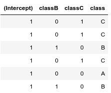
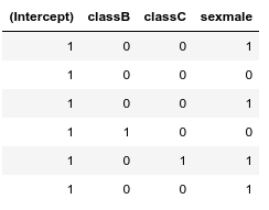
Notice, that if we have more categorical variables, then the baseline ($\beta_0$, intercept) is a combined baseline, in the following example a class A female:
N = 30
sex = sample(c('male','female'),N,replace=TRUE,prob = c(1/2,1/2))
class = sample(c('A','B','C'),N,replace=TRUE,prob = c(1/3,1/3,1/3))
head(model.matrix(~ class + sex))
Fortunately, R takes care of dummy coding, thus if you have a data with both types of variables like what we create in the example below, you can treat them the same, when passing it to the lm (or glm) function:
Input
N = 1000
age = runif(N,20,80)
age = round(age)
group = sample(c('A','B'),N,replace=TRUE,prob = c(1/2,1/2))
temp = runif(N,37,40)
temp = round(temp,digits = 2)

e = rnorm(N,0,1)
recovery = 0.5*age +
           temp +
            model.matrix(~group) %*% c(0.5,1) +
            10 +
            e
recovery = round(recovery,)

df = data.frame("recovery" = recovery,
               "temp" = temp,
               "group" = group,
               "age" = age)
lm(recovery ~ temp + age + group, data = df)
Output
Call:
lm(formula = recovery ~ temp + age + group, data = df)

Coefficients:
(Intercept)         temp          age      groupB
     6.8396       1.0942       0.5001       1.1092
Main factors and interactions
With all this in hand, defining interactions and main effects will be easy. If we have $X_a$ and $X_b$ independent variables, then a linear predictor with an interaction will look like this:
\begin{equation}\eta = \beta_a x_a + \beta_b x_b + \beta_i x_a x_b + \beta_0\end{equation}
where the $\beta_a x_a$ and $\beta_b x_b$ parts are the main effects and the $\beta_i x_a x_b$ is the interaction. If $X_b$ is not a continuous, but a categorical variable, then if there is an interaction between $X_a$ and $X_b$ a new interaction term for each of $X_b$’s dummy coded variable needs to be introduced (but of course R takes care of this).
A note on the R model minilanguage syntax. In Eq. 18 (the mathematical model) the interaction is a multiplication of the two variables $x_a$ and $x_b$, besides having the main effects. In the R model language multiplication (e.g. ~ x_a*x_b) will create both the interaction term and the main effects (and remember, the interaction is also turned on by default), thus ~ x_a*x_b corresponds to the full right side of Eq. 18. To remove the interaction, you need to specify -1 and to only have the interaction, but no main effect, you need to specify x_a:x_b. In the outputs, the coefficient of the interaction ($\beta_i$ in our example) would be denoted by x_a:x_b as well.
aov, anova, Anova in R
Yes, actually, there are basically two things that are called ANOVA. One is doing a linear model with a categorical variable (as we did above), which is done with the aov command in R (which actually calls lm in the background). The other is hypothesis testing based on sum of squares to determine whether the linear predictors we fitted have actual significance to the model or not, which is the anova or the car::Anova function in R.
There is a more in-depth article, aptly titled the “The ANOVA Controversy”, which you can find here.
In summary:
Linear models with a normal distribution and the identity link function:
- ANOVA: categorical explanatory variable
- ANCOVA = general linear model: categorical and continuous explanatory variables
And it’s a generalized linear model if either the distribution is not normal or the link function is not the identity.
Many other things are GLM as well
Originally I wanted to show how some other well known tests are also linear models, but when researching material that, I came across an excellent page by Lindeløv. He does a much better job at it than I planned, with a graphical summary table, non-parametric tests and all, so definitely worth to read!